Bayesian MCMC Site-Level Patient Enrollment Forecasting - Clinical Trial Supply Chain
PyMC3 · Gamma-Poisson Bayesian Inference · AWS Glue · S3 · MLflow · SAP IBP · Veeva Vault
Client: Global Pharmaceutical Client (Top-10 Oncology Biopharma)
Role: ML Engineer & Data Engineering Lead · MLOps Architect
Programme Scale: 8 Phase 2/3 Oncology Trials · 40 Countries · 80+ Trial Sites · 2-Year Delivery
This case study demonstrates core ML engineering principles applicable across any domain requiring probabilistic demand forecasting under extreme data sparsity: Bayesian hierarchical modelling, uncertainty-aware supply planning, and production MLOps for regulated enterprise environments. The model output was adopted at VP level - replacing a methodology that had been in place for over a decade - validating both the technical rigour and the stakeholder engagement approach required to drive change at this scale.
Executive Summary
| Metric | Value |
|---|---|
| Estimated supply waste avoidable over 10 years (model vs 2× heuristic) | ~$2B USD |
| Safety stock heuristic replaced | 2× enrolled patients (over-ordering baseline) |
| Supply planning horizon extended | 3 years (site-level, probabilistic) |
| Forecast accuracy (MAE, monthly) | 63% - first quantitative forecast in client’s oncology trial history |
| Trials monitored | 8 Phase 2/3 oncology trials |
| Geographic coverage | 40 countries |
| Prior method | None - manual heuristic with no ML or statistical modelling |
| Enterprise integration | SAP IBP + Veeva Vault via flat-file pipeline |
This system replaced the client’s 2× enrolled-patient safety stock heuristic - a blunt over-ordering rule that generated $2B of estimated drug and placebo waste over a 10-year horizon - with a probabilistic, site-level, 3-year enrollment forecast grounded in Bayesian inference. For large-molecule oncology drugs in Phase 2/3 blinded trials, where per-patient supply costs are substantial and blinded trial supply requires matched drug/placebo allocation, the reduction in systematic over-ordering had material commercial impact.
The system produced the first statistically grounded supply forecast in the client’s oncology trial history.
1. Business Problem
The Clinical Trial Supply Chain Problem
Pharmaceutical supply chain planning for clinical trials is fundamentally a probabilistic enrollment forecasting problem made structurally harder by:
- Patient attrition: Enrolled patients drop out of trials mid-study due to adverse events, withdrawal of consent, or protocol violations. Dropout rates vary significantly by therapeutic area, site, and country.
- Site-level heterogeneity: Each trial site has a different patient pool, investigator efficiency, country-level regulatory cycle, and activation timeline. A single country-level aggregate forecast masks enormous site-level variance.
-
Blinded trial complexity: For double-blind controlled trials (active drug vs. placebo), drug and placebo must be supplied in matched quantities. Forecast error translates to imbalanced supply for active vs. control arms.
- Long trial durations: Phase 2/3 oncology trials have a 5-year duration. Supply commitments made at trial initiation must be defensible 3 years into the future.
- Irreversible supply decisions: Drug manufacturing lead times make late corrections expensive. Oncology biologics cannot be produced on-demand.
The Heuristic That Was Replaced
The client’s pre-existing approach to trial drug supply was a 2× multiplier on expected enrolled patients: order twice the drug quantity implied by the planned enrollment. This heuristic:
- Did not differentiate by site, country, or therapeutic area
- Made no use of historical site performance data
- Did not account for enrollment velocity - only total planned headcount
- Generated systematic over-ordering estimated at $2B in waste over a 10-year planning horizon
- Provided no confidence intervals or scenario-based planning capability
The Objective
Build a site-level probabilistic enrollment forecasting system that:
- Produces monthly enrollment predictions per site, per country, per trial - with 80% confidence bands
- Accounts for patient attrition and site-level dropout rates
- Handles patient transfers between sites (tracked via IRT reference IDs)
- Updates in real-time as actuals from IRT are observed (Bayesian updating)
- Feeds into SAP IBP for 3-year supply planning, replacing the 2× heuristic
2. Why Bayesian MCMC - Not Classical Forecasting
The Core Challenge: Extreme Data Sparsity at the Right Level of Granularity
The forecasting problem requires site-level, monthly predictions. In practice:
- Oncology trial sites typically enroll 1–5 patients per month
- A given site may have only 3–10 historical observations from prior trials in the same therapeutic area
- Many sites have zero historical data at the indication level - only country-level data exists
Classical time-series approaches (ARIMA, Prophet) require sufficient within-series observations to identify patterns. Site-level enrollment series - with monthly counts of 1–5 patients - violate this requirement entirely.
The Bayesian Advantage
| Requirement | Classical ML | Bayesian MCMC |
|---|---|---|
| Site-level monthly counts of 1–5 | Insufficient signal | ✅ Informative priors encode historical rates |
| Data sparsity at site level | Model collapses | ✅ Prior from country-level observations |
| Uncertainty quantification | Ad-hoc post-hoc CIs | ✅ Native posterior distributions |
| Hierarchical structure (indication → TA → country) | Manual stratification | ✅ Hierarchical prior fallback |
| Bayesian updating with actuals | Requires retraining | ✅ Conjugate posterior update (no retraining) |
| Interpretability for supply chain planners | Black box | ✅ Explicit probabilistic statement |
Why Gamma-Poisson
Patient enrollment at a site is naturally modelled as a Poisson process: patients arrive independently at a rate λ (patients per month). The Poisson parameter λ itself is site-specific and uncertain - modelling λ as a Gamma-distributed random variable gives the Gamma-Poisson (Negative Binomial) compound distribution, which:
- Accommodates overdispersion in real enrollment counts
- Provides a conjugate prior-posterior structure enabling closed-form Bayesian updates
- Produces natural 80% credible intervals aligned to supply planning needs
3. Data Architecture & Engineering
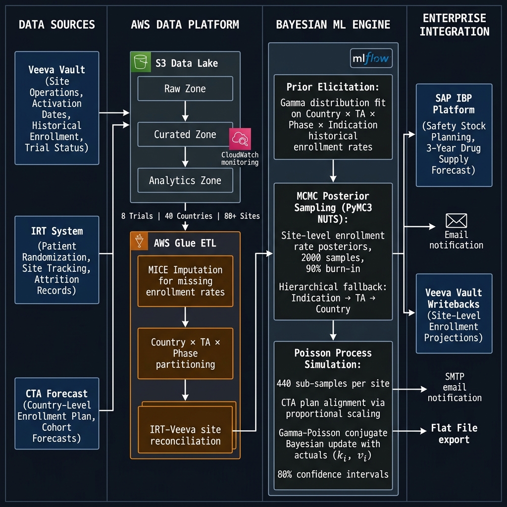
Data Sources
| Source | System | Contents |
|---|---|---|
| Veeva Vault | Clinical Operations | Site activation dates, site status, historical enrollment rates (MICE-imputed), trial metadata, TA/Phase/Indication classification |
| IRT System | Interactive Response Technology | Patient randomisation records, site-level monthly actuals, patient tracking IDs, dropout reason codes |
| CTA Forecast | Clinical Trial Agreement | Country-level planned enrollment curve (Cohort-0 baseline), monthly expected totals |
AWS Data Platform
The data engineering architecture was designed and operated on AWS:
- Amazon S3: Three-zone data lake - Raw (source replication), Curated (validated, schema-enforced), Analytics (partitioned by country × protocol × site)
- AWS Glue: ETL pipeline executing:
- Source-system schema normalisation across Veeva, IRT, and CTA formats
- MICE (Multiple Imputation by Chained Equations) for missing enrollment rate imputation - critical because many historical trial sites have sparse records
- IRT-Veeva site reconciliation (matching IRT site IDs to Veeva site IDs via trial metadata joins)
- Country × TA × Phase × Indication partitioning for prior computation
- Monthly incremental refresh aligned to IRT update cadence
- Amazon CloudWatch: Pipeline execution logging, data quality alerts, SLA monitoring for monthly batch jobs
- SMTP: Automated email notifications to trial operations teams on forecast completion and model alerts
IRT-Based Patient Transfer Tracking
A non-trivial data engineering challenge: patients occasionally transfer between sites. Without correction, a transferred patient appears as a dropout at the source site and a new enrollment at the destination - inflating attrition and enrollment rates simultaneously.
Resolution: IRT stores a patient tracking ID and a reason-for-dropout field. By joining on tracking IDs across site records within a protocol, transfers were identified and excluded from attrition counts, with enrollment credited to the correct receiving site. This required building a patient-level reconciliation layer in Glue above the site-level aggregation.
4. Modeling Architecture
Overall Design: Two Operating Modes
┌────────────────────────────────────────────────────────────┐
│  MODE 1: BASELINE FORECAST (Trial in Planning Stage)       │
│  Inputs: Veeva (historical) + CTA plan                     │
│  Output: Site-level enrollment projections from t=0        │
│  → Country_Forecast_Adaption.py                            │
├────────────────────────────────────────────────────────────┤
│  MODE 2: REFORECAST (Trial Active, IRT Actuals Available)  │
│  Inputs: Veeva + CTA plan + IRT actuals                    │
│  Output: Updated projections incorporating observed data   │
│  → Reforecast.py (Bayesian conjugate update)               │
└────────────────────────────────────────────────────────────┘
Step 1 - Prior Elicitation (Country-Level Distribution Fitting)
For each Country × TA × Phase combination, historical enrollment rates from completed or closing trials (excluding the current protocol) were extracted. A Gamma distribution was fit to these rates using maximum likelihood estimation (SciPy):
# Fit Gamma distribution to country-level historical enrollment rates
a, loc, scale = gamma.fit(data=metric_observed_values, floc=-1e-10)
param_dict = {'alpha': a, 'beta': 1/scale, 'loc': loc}
Two prior variants were generated per site:
- Indication-level prior: filtered to matching indication (e.g., solid tumour oncology)
- TA-level prior: filtered to therapeutic area only (broader, used as fallback)
Step 2 - MCMC Posterior Sampling (Site-Level, PyMC3)
For each site with historical observations, the Gamma prior was updated against site-level observed enrollment rates using MCMC posterior sampling via PyMC3 with the NUTS (No-U-Turn Sampler):
with pm.Model() as mcmc_model:
    # Informative Gamma prior from country-level distribution
    alpha = BoundedNormal('alpha', mu=alpha_mean, sigma=1, testval=10)
    beta  = BoundedNormal('beta',  mu=beta_mean,  sigma=1, testval=10)

    # Likelihood: enrollment rate is Gamma-distributed
    observed = pm.Gamma('obs', alpha=alpha, beta=beta,
                        observed=site_enrollment_rates)

    trace = pm.sample(2000, step=pm.NUTS(), chains=2, tune=200)

# Use final 10% of chain (post burn-in) for posterior estimates
alpha_posterior = trace['alpha'][int(0.9 * n_samples):]
beta_posterior  = trace['beta'][int(0.9 * n_samples):]
Hierarchical Fallback Logic (handles cold-start sites):
Site has indication-level data?
  └─ YES → MCMC update with indication-level prior
  └─ NO  → Site has TA-level data?
              └─ YES → MCMC update with TA-level prior
              └─ NO  → Sample directly from country-level Gamma prior
Step 3 - Poisson Process Simulation
With each site’s posterior Gamma parameters, enrollment trajectories were simulated using an inverse-method Poisson process:
# Simulate patient inter-arrival times (inverse Poisson)
inter_event_time = -log(1 - uniform_random) / lambda

# Run 440 independent sample paths per site
# Generates monthly enrollment counts over the forecast horizon
This simulation naturally captures the discrete, stochastic nature of patient arrivals - months with zero patients, burst months, and long-term variance are all represented in the sample paths.
Step 4 - CTA Plan Alignment
Raw MCMC-derived site rates are anchored to the country-level CTA forecast. The adjustment:
- Compute each site’s proportional share of the country-level MCMC enrollment rate
- Compute the residual between the CTA plan and the sum of all site MCMC rates
- Distribute the residual to each site proportionally - preserving site rankings while ensuring country totals match the agreed CTA plan
psm_ratio = mean(site_samples) / country_level_mean
site_adjusted = site_samples + (psm_ratio * cta_residual)
Step 5 - Reforecast: Bayesian Conjugate Update
Once trials are active, IRT actuals enable a Bayesian posterior update without re-running MCMC:
Given:
k_i= patients actually enrolled at site i (from IRT)v_i= months the site has been active (from activation date to current month)- Prior:
Gamma(α, β)
→ Conjugate posterior: Gamma(α + k_i, β + v_i)
This is exact Bayesian updating for a Gamma-Poisson model. The posterior becomes the new sampling distribution for Poisson process simulation over the remaining forecast horizon.
Confidence Interval Construction
80% confidence intervals were computed via t-distribution over the 440 sample paths per site:
t_val = t.ppf((1 + 0.80) / 2, df=10000)  # ~1.282
lower = max(0, mean_enrollments - t_val * std_enrollments)
upper = mean_enrollments + t_val * std_enrollments
5. MLOps & Model Governance
Model Tracking
Model runs were tracked in a proprietary MLOps platform with MLflow-based model tracking:
- Per-trial, per-country experiment tracking
- Prior parameter snapshots (Gamma α, β per site) stored as artefacts
- MCMC trace artefacts for audit and reproducibility
- Model version registry aligned to trial protocol IDs
Inference Pipeline (Batch)
The system operated as a monthly batch pipeline:
Monthly Trigger
    → AWS Glue: Extract IRT actuals, refresh S3 Curated zone
    → MCMC: Re-sample posteriors for active sites (actuals updated)
    → Reforecast: Run Poisson process simulations (440 samples × N sites)
    → Output: Flat-file per trial (site × month × mean/low/high)
    → Delivery: SMTP notification + flat file to SAP IBP staging
The flat-file integration to SAP IBP was a deliberate design choice: IBP has a defined intake schema for supply plan inputs, and a file-based interface decoupled the ML system from IBP’s internal release cycles while maintaining auditability of every number that entered the supply plan.
Monitoring & Alerting
- CloudWatch for Glue job health, data freshness SLA, and pipeline completion
- SMTP alerts to trial operations teams on: forecast completion, data quality flags (missing IRT uploads, Veeva schema changes), and sites flagging implausible enrollment velocity
6. Cross-Functional Delivery
This programme required orchestration across 15 people spanning 4 organisations:
| Workstream | Organisation | Responsibility |
|---|---|---|
| ML Modelling | Client / Vendor | Bayesian model design, MCMC implementation |
| Data Engineering & MLOps | Client | AWS Glue pipelines, S3 data lake, MLflow governance |
| Clinical Operations | Client | Veeva data ownership, IRT configuration, trial metadata |
| Supply Chain Planning | Client | SAP IBP integration, safety stock methodology, demand signals |
My direct team (4 engineers + self) owned: AWS data pipelines, S3 lake architecture, Glue ETL, MLflow model governance, flat-file IBP integration, CloudWatch monitoring, and end-to-end delivery coordination.
Programme delivery: 2 years from requirements to production - requirements definition, data architecture design, Glue pipeline build, model integration, SAP IBP integration, and trial operations team training.
Stakeholder engagement: Programme success metrics were reviewed with Supply Chain VP and Clinical Operations leadership on a quarterly basis. The decision to integrate model outputs into SAP IBP as the system of record for safety stock planning was made at VP level - replacing a methodology that had been in place for over a decade.
7. Domain Complexity: Blinded Trial Supply
For blinded, controlled oncology trials (e.g., active drug vs. placebo), supply planning has an additional constraint: the drug-to-placebo ratio must be maintained at the site level throughout the trial to preserve blinding. This means:
- Enrollment forecasts must feed two supply plans (active drug + matched placebo)
- Attrition affects both arms - but if one arm has higher dropout, imbalance can compromise blinding
- The confidence interval on enrollment directly determines the safety stock buffer for each supply arm
The system produced separate enrollment projections for each trial arm via the site-level outputs - allowing supply planners to calculate arm-specific safety stock quantities in SAP IBP rather than applying a blanket 2× multiplier to total trial enrollment.
8. Results & Business Impact
Quantitative Outcomes
| Outcome | Value |
|---|---|
| Forecast accuracy (first-ever quantitative forecast) | 63% MAE - monthly site-level |
| Estimated supply waste eliminated | $2B over 10-year planning horizon |
| Safety stock heuristic | Replaced: 2× enrolled-patient blanket rule → probabilistic 80% CI |
| Planning horizon | Extended from reactive to 3-year forward-looking |
| Trials operationalised | 8 Phase 2/3 oncology trials |
| Countries covered | 40 countries |
| SAP IBP integration | Monthly batch · flat-file · automated |
Why 63% Is a Strong Result
In clinical trial enrollment forecasting, 63% MAE accuracy at the monthly site level is a materially strong result given:
- Site-level monthly enrollment counts of 1–5 patients are inherently low-signal and noisy
- Oncology trials have high and unpredictable attrition (adverse events, disease progression)
- 40 countries introduce country-level regulatory and operational heterogeneity
- No benchmark existed - the client had never quantitatively forecast at this level before
The relevant comparison is not 63% vs. 90% - it is 63% vs. 0% (the prior state: a fixed 2× heuristic with no forecast capability at all).
The $2B Impact Logic
The 2× safety stock heuristic was shown to systematically over-order relative to actual enrollment. For oncology biologics:
- Per-patient supply cost is substantial (drug manufacture + cold chain + wastage)
- Matched placebo adds a parallel manufacturing cost
- Expired or unusable trial drug is written off
- Across 10 years of Phase 2/3 programme spend at this scale, the model-derived supply quantities showed the 2× buffer generated approximately $2B in avoidable waste
9. Technical Alternatives Evaluated and Rejected
| Alternative | Reason Rejected |
|---|---|
| Prophet / ARIMA | Monthly site-level series of 1–5 events: insufficient for time-series pattern identification |
| XGBoost regression | No native uncertainty quantification; requires large training dataset per site |
| Simple Gamma MLE (no MCMC) | No posterior uncertainty; point estimate doesn’t propagate to supply confidence intervals |
| Neural Bayesian (e.g., Pyro) | Overkill for data volume; NUTS convergence preferable at this problem scale |
| Single country-level forecast disaggregated proportionally | Cannot capture site-level activation timing or site-specific attrition patterns |
10. Lessons Learned
- Conjugate Bayesian updating is operationally underrated. The Gamma-Poisson conjugacy meant that mid-trial reforecasting required no MCMC re-run - just an arithmetic posterior update with new actuals. This reduced monthly reforecast compute cost dramatically and made the monthly cadence operationally viable.
- IRT-Veeva reconciliation was more complex than anticipated. Site IDs in IRT and Veeva used different reference systems and update cadences. Building the patient-transfer deduplification layer (tracking ID join + reason code filter) was a 3-month engineering effort that fundamentally changed attrition accuracy.
- CTA plan alignment is essential for adoption. Supply planners trust their CTA plan above all. An MCMC forecast that ignores the CTA agreement will not be adopted. The proportional scaling step that anchors site-level predictions to the country-level CTA forecast was the key design decision that enabled clinical operations buy-in.
- Enterprise integration is the last 30% of the work. The ML model was complete months before production. The flat-file SAP IBP integration, Veeva writeback, CloudWatch alerting, and trial operations team training consumed as much engineering effort as the modelling itself.
- What I’d approach differently today: A full hierarchical Bayesian model (PyMC with pooled country-level hyperpriors) would eliminate the manual fallback cascade (indication → TA → country) and allow partial pooling across sites. I’d also explore Sequential Monte Carlo (SMC) for real-time reforecasting as IRT actuals arrive, rather than the monthly batch update cadence.
- Cross-domain note for engineering audiences: The key abstraction here is that the Bayesian conjugate update step replaces a full model retrain. This pattern - maintain a prior, update with actuals, re-simulate - applies to any supervised setting where you want online adaptation without retraining pipelines. The same principle drove our fast iteration on the GenAI cost-governance layer at Tredence.
System Architecture
Technology Stack
| Category | Technology |
|---|---|
| Bayesian Inference | PyMC3 · NUTS Sampler · Metropolis-Hastings |
| Statistical Modelling | SciPy (Gamma MLE) · NumPy · Pandas |
| Data Engineering | AWS Glue · Amazon S3 (3-zone lake) |
| Imputation | MICE (Multiple Imputation by Chained Equations) |
| ML Governance | MLflow (experiment tracking · model registry · artefacts) |
| Orchestration | AWS Glue Workflow · CloudWatch Events |
| Monitoring | Amazon CloudWatch · SMTP alerts |
| Enterprise Integration | SAP IBP (flat-file) · Veeva Vault |
| Clinical Data Systems | Veeva Vault · IRT (Interactive Response Technology) |